This post on Computational Fluid Dynamics (CFD) continues the series of posts dedicated to the CFD simulation of scenarios where turbulence plays a fundamental role. In this case, we discuss the importance of defining flow inlet conditions that accurately represent reality.
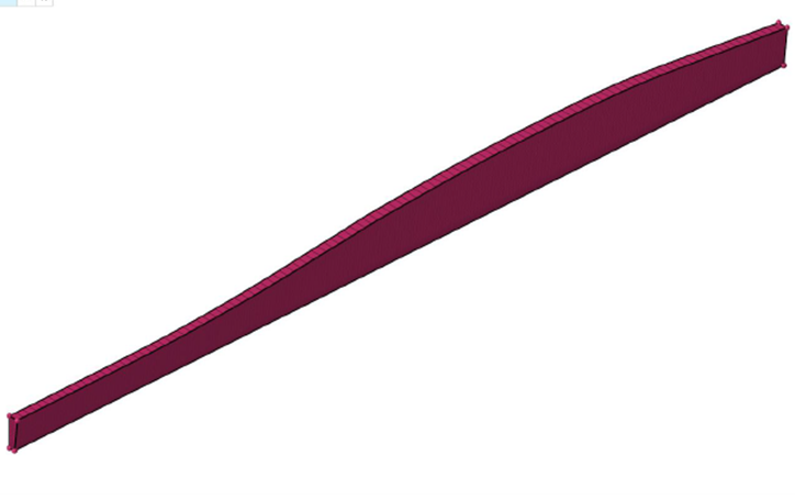
We work again with a practically two-dimensional domain as the device has a clear symmetry in cylindrical coordinates. In this case we will work with Hyperworks CFD to prepare the model and we will solve it using Acusolve. The geometry of the simulation domain can be seen in the following image.

Model preparation and definition of input conditions
The objective will be to compare the results of various turbulence models with a set of experimental data. The inlet conditions in the real case are not uniform, but for the CFD simulations we will give an estimate of the average conditions at the inlet.
In this way, we can check whether the results obtained are in line with reality with this simplification or whether it would be necessary to define a more complex and realistic distribution before launching the simulation. The models to be compared are SST, K-omega, Realisable K-Epsilon and Standard K-Epsilon.
CFD Simulation and Results
The full results can be found in our Downloads section. Some results are also available in Ansys Fluent where the conditions at the inlet have been placed directly by importing a profile of the magnitudes at the inlet. The following is an example of the velocity results using the SST model in Acusolve.

Analysis of results
To compare the results obtained by CFD simulation with the experimental results, a similar process as in the previous tutorial is carried out. Point probes are placed along the centreline of the bottom wall and at certain other locations. These measurements are exported to a spreadsheet where the results are processed to generate graphs.
Some representative coefficients and velocity profiles at certain sections are calculated using their definitions. These are compared with experimental results. As an example, the graphs of the friction and pressure coefficients are shown below.

In this case it is found that the friction coefficient fit can be improved, especially in the inlet area, but once the flow develops it becomes acceptable, especially with the Realisable K-Epsilon model.
As for the pressure coefficient, the fit is remarkably poor throughout the domain. This is due to the fact that the definition of the pressure coefficient takes the representative pressure of the inlet as the value for the dimensioning. Therefore, the error of the mean approximation at the inlet is greatly amplified.
From this study it can be concluded that it is essential to know the flow properties at the inlet before launching a CFD simulation, especially if numerical values of the flow beyond the global behaviour are desired. In case these properties cannot be estimated faithfully, the domain must be generated in such a way that the results of interest are sufficiently far from the inlet.


