In this new entry on Computational Fluid Dynamics (CFD) we are going to simulate the external aerodynamics of a NACA 0012 airfoil. For this study we will also use Acusolve with Hypermesh and Hyperworks CFD preprocessors. In this field of CFD studies, Acusolve has a particularly extensive documentation and validation.
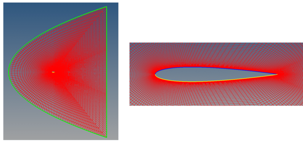
The geometry of the profile together with many other experimental data can be easily found in the bibliography. The study starts in this case from a mesh previously made with Ansys Fluent, which can be seen in the image imported into Hypermesh.
All the steps to follow from importing the mesh to obtaining results are detailed in a tutorial available in our Downloads section.
Pre-processing with Hyperworks CFD and Hypermesh for Aerodynamics
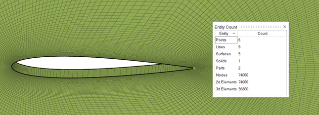
For this type of problem, where we start from a mesh made in other software, we propose two different solutions. The first one follows the approach of the previous tutorials and is based on using only Hyperworks CFD starting from the geometry to build the model. The second and more recommended solution is to use Hypermesh to work directly with the mesh provided. The results shown at the end of the post correspond to the second method. In either case, to capture well the phenomena that occur in this type of flow, the area near the airfoil must be meshed with very fine elements.
The following image shows the model already built within Hyperworks CFD together with the summary of mesh characteristics.
Resolution and Post-processing
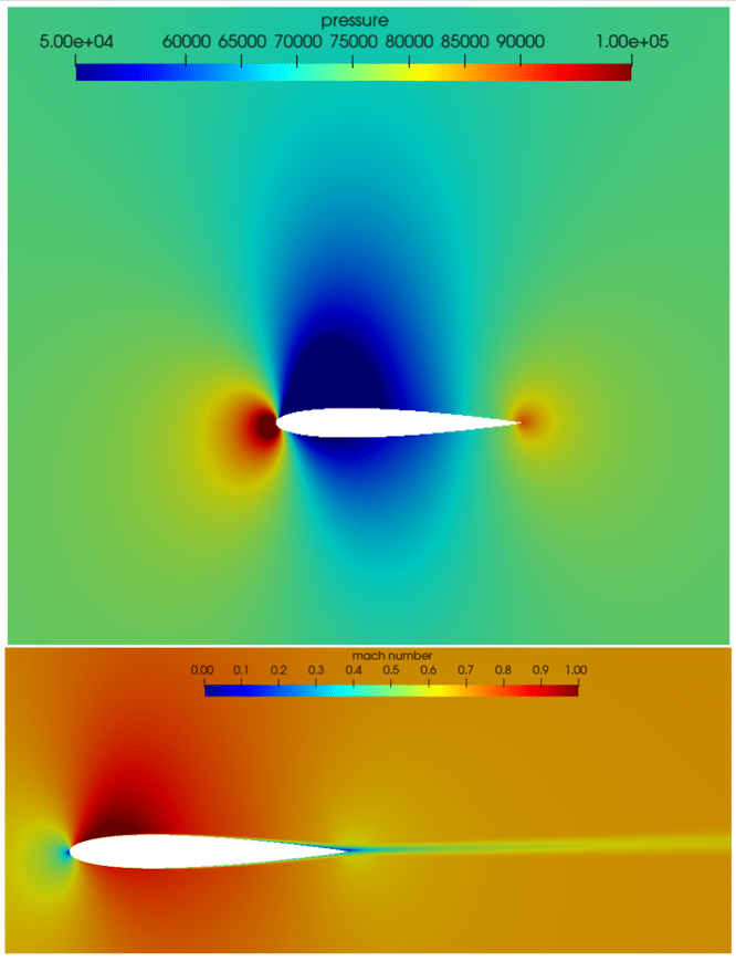
The Acusolve simulation works with the compressible flow equations and provides all the results of interest in this type of study. The following images show the pressure profiles and Mach number after letting the software perform 1000 iterations. In general, this type of aerodynamic analysis usually requires quite a few iterations to reach a clear convergence in the numerical results of interest.
Finally, the tutorial shows a study of the lift and drag coefficients of the airfoil using the “AcuLiftDrag” tool included in the Acusolve software. Simulation results are provided to perform the calculation. These are compared with experimental results, showing relative errors of less than 4% in both cases.
